This post was written after reading and being inspired by Kevin Systrom’s (co-founder of Instagram) post: The Metric We Need to Manage COVID-19
The post talks about using the $R_{0}$ and $R_{t}$ values to predict the spread of an epidemic, in current context the spread of covid-19 in NYC.
I was intrigued by how these values are calculated and what is the intrinsic model that drives these calculations. That’s when I came across the SIR model. This is the first of many posts to come regarding the SIR model and $R_{0}$ and its relation to the covid-19 and India.
What is the SIR model? Link to heading
The SIR model is used to depict how a particular disease may spread. The model is built over diseases which you can only contract once i.e. if you build immunity towards such diseases you’re not going to catch it again. This goes for diseases such as smallpox, polio, measles, and rubella. This is also the same reasoning about having vaccines for the mentioned diseases.
Building a basic SIR model Link to heading
To understand the model, there are a few assumptions to be made
- The population fits into one of these three categories:
- Susceptible (S): those who can catch the disease
- Infectious (I): those who can spread the disease
- Removed (R): those who are immune and cannot spread the disease
- The population is large but fixed in size and confined to a well-defined region.
- The population is well mixed; ideally, everyone comes in contact with the same fraction of people in each category every day.
The disease is no longer a problem when the number Infectious goes to zero. Apart from this, it can be seen that the flow of people is as follows:

So for a particular disease, a person recovers after being infected for X days. This means that if I is the number of people infected on day t, then $\frac{1}{X}I$ is the number of people who recover the next day. i.e.
$$R_{t+1} = R_{t} + R_{t\new}$$ $$R{t\_new} = \frac{1}{X}I$$
Therefore since $\frac{1}{X}I$ is a constant for a given disease; we can set:
$$ b = \frac{1}{X}I$$ $$ R_{t\_new} = bI$$
Here b is how quickly people recover. For e.g. $b = \frac{1}{X}I$ for rubella, since a person suffering from rubella takes on average 11 days to recover.
Next we identify the number of people that each infected person from this population comes in contact with for the entire infection period. Let’s name this variable c.
c = the average number of contacts per infective during the whole infectious period
This will include people from S, I, R. How do we measure c? That’s for later, for now let’s assume it’s a constant.
The number of contacts per infective day is given by a = b * c as b is (1 / number of infection days) and c is the total infection period.
Putting this together we can now derive the total number of adequate contact per day (number of people that infective people come in contact with).
a * I = number of adequate contact
But only people who are Susceptible can become infectious, hence we can define the number of new cases per day:
new cases per day = $a \\frac{S}{N} I$
Where N is the total population, N = S + I + R.
Putting it together Link to heading
b = 1 / Average number of days infectious
c = Average total number of contacts per infective
a = Contacts per infective day
N = Total number of people
So per day increments can now be calculated:
$$\Delta S = - a \frac{S}{N} I$$ $$\Delta I = a \frac{S}{N} I - bI$$ $$\Delta R = bI$$
We can simplify this by denoting:
$$\Delta S = - a \frac{S}{N} I$$ $$∆R = bI$$ $$∆I = -∆S - ∆R$$
Notice that while the number of people who move from S -> I is the same, people also move from I -> R.
Example Link to heading
Let’s consider an example to solidify our thoughts. Let’s consider the spread of rubella through an imaginary city.
We know that number of days to recover from rubella is 11 days. Therefore b = 1⁄11. Let’s consider a case where at t0 the values are as follows:
$$S = 25000$$ $$I = 1000$$ $$R = 4000$$
For our population let’s assume c = 6.8.
We know a = b * c therefore a = $\frac{1}{11} 6.8$ = 0.618.
Using this, let’s plot the data for the next t days.
|
|
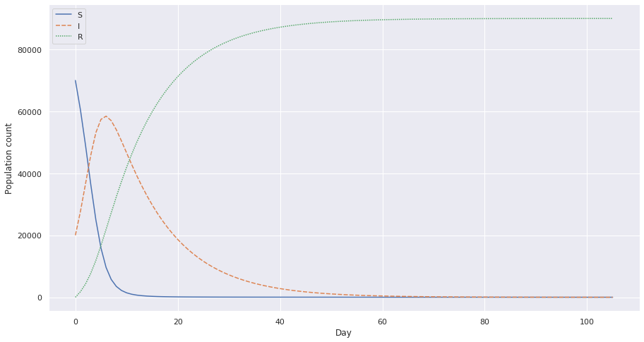
This shows how the spread is when c = 6.8. Notice how the the I value peaks very fast? This is bad because it strains the population with a lot of cases in very short amount of time. This would put a stress on the health facilities of the population.
Let’s try with a decreased c value. Which is possible when the population undergoes preventive measures such as social distancing. Let’s see the plot for c = 3.9, which is half the previous value.
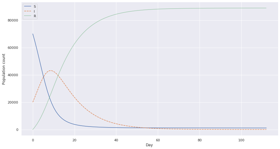
Notice the crest and how it’s flattening a little more and how instead of rapidly increasing I, we have a flatter slope.
This is a plot with c = 1.95, 1⁄4th the initial value.
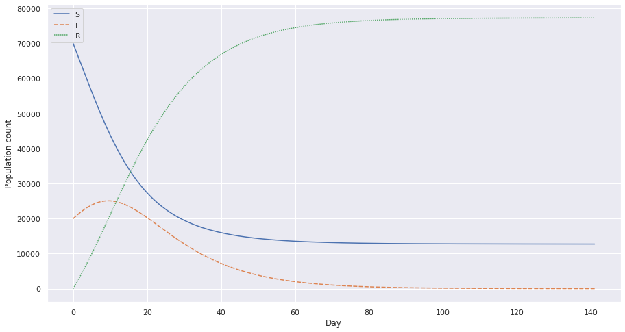
These graphs give us an idea of how we can effectively decrease the load of a disease and lower the numbers with simple preventive measures.
Credit Link to heading
I mostly referred to these resources while writing this blog post:
https://homepage.divms.uiowa.edu/~stroyan/CTLC3rdEd/3rdCTLCText/Chapters/Ch2.pdf
https://en.wikipedia.org/wiki/Compartmental_models_in_epidemiology